Perception & Cognition (PSYC2071)

Physical aspects

First, we need to consider the physical side — what are the physical characteristics of the stimulation we are investigating?

We will concentrate on visual motion as our example physical stimulus. We can start by defining motion:

Motion

A change in the position of a feature in a visual pattern over time.

The capacity to represent the motion that is present in visual input is fundamental for many biological systems, and we have talked (or will talk) about motion processing in detail in lectures.

Random-dot motion

The perception of motion is often explored using a class of stimuli known as "random dot kinematograms". To make such a stimulus, we place a large number of small circles (called 'dots') at random positions within the image. Then, we change the position of each dot over time to produce a moving stimulus.

An example of such a stimulus is shown below. If you left-click on the play icon (▶), you will see all the dots move in a particular direction (rightwards, in this case).

As has been the case in many of the demonstrations in this course, the videos in this tutorial contain high-contrast flicker. Please be cautious with your viewing if you have a hypersensitivity to such stimulation.

Why does the video look like it is 'flickering'? Because we want our definition of motion to encompass the whole stimulus and not just individual dots, each dot is only present in the video for a short time (around 150-200 milliseconds) before being replaced by a new dot in a random position. This continual re-generation of the dot positions is what gives the 'flicker'.

Space-time representations

We can think of the above video as having three dimensions — horizontal space, vertical space, and time. However, it is often convenient to visualise just two of these dimensions rather than all three. These sorts of figures are known as space-time representations.

For our example video above, let's ignore the vertical dimension of space by extracting just one row — that is, just one horizontal slice. Here, we will only consider the row that is at the vertical centre of the video. We can then visualise how the intensities across this one row change over time — this is the space-time representation shown below:

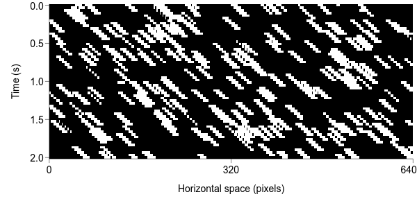
These space-time representations can be difficult to interpret at first, so let's walk through the above figure:

• The horizontal axis represents horizontal space in units of pixels, with 0 corresponding to the leftmost edge of the video, 320 corresponding to the centre of the video, and 640 to the rightmost edge of the video (the video's horizontal 'resolution' is 640 pixels).
• The vertical axis represents time in units of seconds, with 0 (at the top of the axis) corresponding to the start of the video and 2 corresponding to the end of the video.
• Each location on the graph thus represents the video intensity at a particular horizontal point in the centre vertical row of the video (remember that we limited ourselves to only looking at the central vertical row) at a particular point in time.

Why are space-time representations useful?

The neat thing about this form of representation is that the properties of the motion can be evident in the static form of the space-time depiction. That is, rather than needing to watch a video, we can just look at an image to be able to figure out what sort of motion would be present in the video.

For this example, we can see that whenever we have a point of high intensity (white) at a particular point in time, the horizontal location of that point of high intensity is shifted rightwards at the next point in time — producing a series of down-and-to-the-right 'streaks' in the space-time representation. Hence, we can infer that there is likely to be rightwards motion in the video.

It is important to highlight a common misconception here. The space-time plot shown in the does not show that the motion is moving 'down and to the right'. Because we have limited ourselves to one spatial dimension only (horizontal), we cannot infer motion in the vertical direction from the space-time plot. Remember, the vertical axis is time.

Controlling motion strength

If asked to describe the motion in the video, nearly all observers would be able to perform the task perfectly — that is, they would say that they see a set of dots moving rightwards. Because the properties of the physical stimulation are such that it is very easy for us to perceive, detailed measurements of behaviour would not be very informative.

A common way to probe motion sensitivity is by describing the visual stimulus in terms of its global motion direction and its coherence. These terms are defined as:

Global motion direction

The common direction of motion for a particular subset of dots in the stimulus.

Coherence

The proportion of dots that move in the global motion direction.

Let's reconsider the first example we saw, shown again below:

With this new terminology, we can describe this stimulus as having a "rightwards global motion direction and a coherence of 100%". This is because all of the dots are moving in the same direction (so 100% coherence), and that direction is rightwards (so a rightwards global motion direction).

Now, we can control the 'strength' of the global motion by changing the coherence. In the video below, half of the dots are moving rightwards and the remainder are moving in random directions. This is a change in coherence — this example has a coherence of 50%, because half of the dots are moving in the global motion direction.

Left-click on the play icon (▶)in the video below to see the example of a stimulus with 50% coherence.

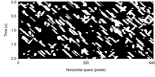
As you can see, the perception of a global motion direction has become somewhat 'noisy'. This 'noisiness' is reflected in the space-time representation of the 50% coherence sequence. As shown in the figure below, the pristine down-and-to-the-right streaks of the 100% coherence stimulus have been corrupted by other blobs of intensity in this 50% coherence stimulus.

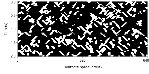
We are quite good at detecting coherent global motion so it is likely that you are still able to pick out the rightwards motion in the above example. Let's try it at 5%:

Again, the increased levels of noise are visible in the space-time representation, as shown in the figure below:

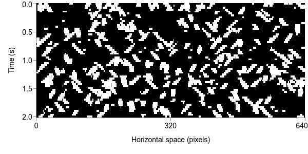
Finally, we can remove the coherent global motion altogether by setting the coherence to 0%. That is, each dot is moving in its own random direction so there is no overall global motion coherence. As we will see, this is an important stimulus when we begin incorporating the psychological dimension and measuring perceptual sensitivity.

Left-click on the play icon (▶) in the video below to see an example of a 0% coherence stimulus.

As expected, there is little structure evident in the space-time representation, as shown below:

Summary

The first step in a psychophysical investigation is to consider the physical stimulation. Here, we investigated the stimulus attribute called motion and its implementation in random-dot kinematograms. We saw how motion can be visualised in space-time representations and how defining the physical stimulus in terms of its global motion direction and its coherence allows us to vary the strength of the physical signal.

Next, we will introduce the psychological aspect of measuring perception within a framework called signal detection theory.